In our previous blog post, we covered one of the first steps in creating a fully beneficial actuarial analysis. With that out of the way, let’s walk through another crucial step in the process: the calculation of loss development factors.

It may take several years for all claims in a given policy period to be completely paid and closed. New information pertaining to existing claims could impact the total losses long after the end of a policy period, and claims occurring during the policy period may be reported after it expires. As such, a snapshot of losses made at the end of the policy period and at each subsequent year provides a good indication of how losses develop from year to year.

The loss development triangle is a unique way of arranging these annual snapshots for past policy periods. The standard format is shown below. Notice that losses are arranged in each column according to the length of time between the beginning of the policy period and the snapshot’s evaluation date. By arranging the loss data in this way, we can easily analyze the change in losses from one evaluation to the next.

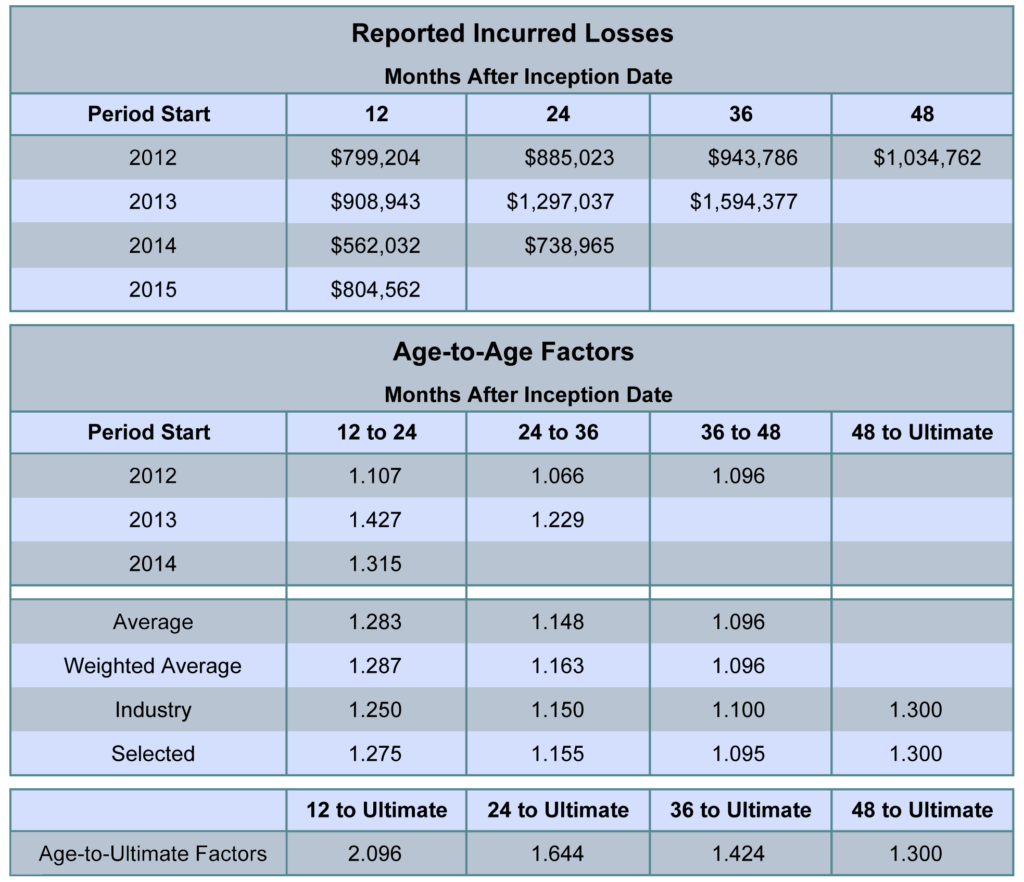
The rates by which losses develop from one evaluation to the next are calculated by dividing losses in each column by losses in the prior column for each historical policy period. For example, the table above lists the 12 to 24 age-to-age factor for the 2007 period to be 1.427, which is the 24 month incurred amount of $1,297,037 divided by the 12 month incurred amount of $908,943. A loss development factor calculated to be less than 1.000 indicates that the value of reported losses declined, possibly due to a claim being settled for an amount less than was previously reserved.

Several averages of age-to-age factors are then calculated and shown alongside industry figures in order to select factors most representative of expected loss development. Computation of loss development factors is based on the selected age-to-age factors. The 12 month to ultimate loss development factor, for instance, is found by multiplying the 12 to 24 month age-to-age factor by the 24 month to ultimate loss development factor.

A number of industry sources exist for loss development factors, such as the National Council on Compensation Insurance (NCCI), state rating bureaus, or Best's Aggregates and Averages. In some cases, either industry factors or a blend of unique and industry factors may be used. However, the use of unique loss development factors typically results in higher accuracy, provided the historical database is stable and credible.

The development factors to be applied to reported losses are selected based on the time elapsed from the beginning of the loss period and the date of the most recent evaluation. In most cases, the closer the evaluation date is to the period effective date, the larger the loss development factor needed. Conversely, as the period matures, the loss development factor approaches 1.000. Expected ultimate losses for each period are estimated by multiplying the applicable development factor by the period’s recently valued reported losses.

This blog post has hopefully given you a better understanding of loss development factors, but quite a bit more nuance surrounds their creation and use. Below are links to a few relevant RISK66 documents and videos that provide a deeper investigation.

TechTalk Article: Understanding Loss Development Factors
Video: Loss Development Factors
Video: Loss Development Triangles

As always, feel free to contact us with any questions regarding loss development factors, and we’d be more than happy to discuss them. We hope you’ll join us for our next post as we combine our knowledge on the past two topics and focus on one of their primary uses: reserve and cash flow analyses.