Trending to the Future

In a prior blog article, we discussed loss development factors and IBNR analysis. The IBNR analysis includes the estimation of ultimate incurred losses for past years, but what about future years? If we also have an estimate of exposures, then we can compute pure loss rates (trended losses per some unit of trended exposure) which can ultimately be used to forecast losses for the coming period. For workers compensation, the most common exposure to analyze is payroll. Other lines of coverage use other exposures. For example, general liability may use sales or square footage. Automobile liability may use number of vehicles or miles driven.

The estimated ultimate incurred losses and the exposures must be trended, or adjusted for inflation, to today’s dollars before pure loss rates are computed. Noninflationary exposures, like vehicle counts, do not need to be trended.

Inflation trend factors are applied to historical incurred losses to more accurately reflect the expected cost level for the period being projected. The historical losses are adjusted from each period to the midpoint of the projected period. In the set of factors for workers compensation shown in Figure 1a, the factor of 1.152 for the 1/1/14 period indicates an increased average loss cost of 15.2 percent. These factors include changes in workers compensation benefit levels, indemnity trends and medical cost trends. You may see the term BLCF (Benefit Level Change Factor) in some actuarial reports. This factor, which quantifies increases in benefit levels attributable to changes in state workers compensation laws, is developed from individual state data. The medical factor is an inflation rate for medical costs. The indemnity factor is a wage inflation rate that reflects the inflation in the indemnity portion of the claim. The term “severity factor” may also be used to describe the medical and indemnity trend factors. The combination of all these inflation rates results in the inflation trend factor. For a liability coverage, the trend factor is based on changes in loss costs over time.

Once the trended losses and exposures are calculated, the final step, selecting a pure loss rate, requires a portion of judgment. In order to better understand this process, we will walk through a sample case involving workers compensation.

Sample Case – Trending Historical Losses and Exposures

Figures 1a and 1b show tables which reflect the trending steps in a typical actuarial analysis.

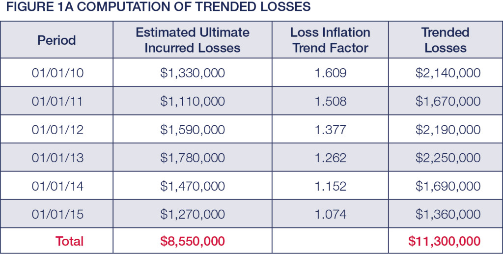
Figure 1a shows the estimated ultimate incurred losses and the loss inflation trend factor for past years. The trended losses for each year are then computed as the estimated ultimate incurred losses multiplied by the trend factor for that year.

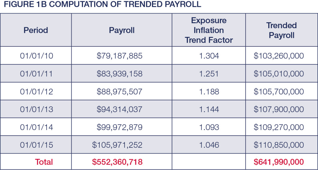
Having trended the historical losses in Figure 1a, the next step is to trend historical exposures to appropriate expected levels for the projected period. In this example, the exposure inflation trend factors are based on average hourly wages as measured by the United States Department of Commerce. Historical payroll amounts are adjusted to anticipated average wage levels for the projected period.

In Figure 1b, the exposure base (payroll in this case) is shown along with the exposure inflation trend factor. The trended exposures are then computed as the payroll multiplied by the trend factor for each year.

Sample Case – Computing the Pure Loss Rates

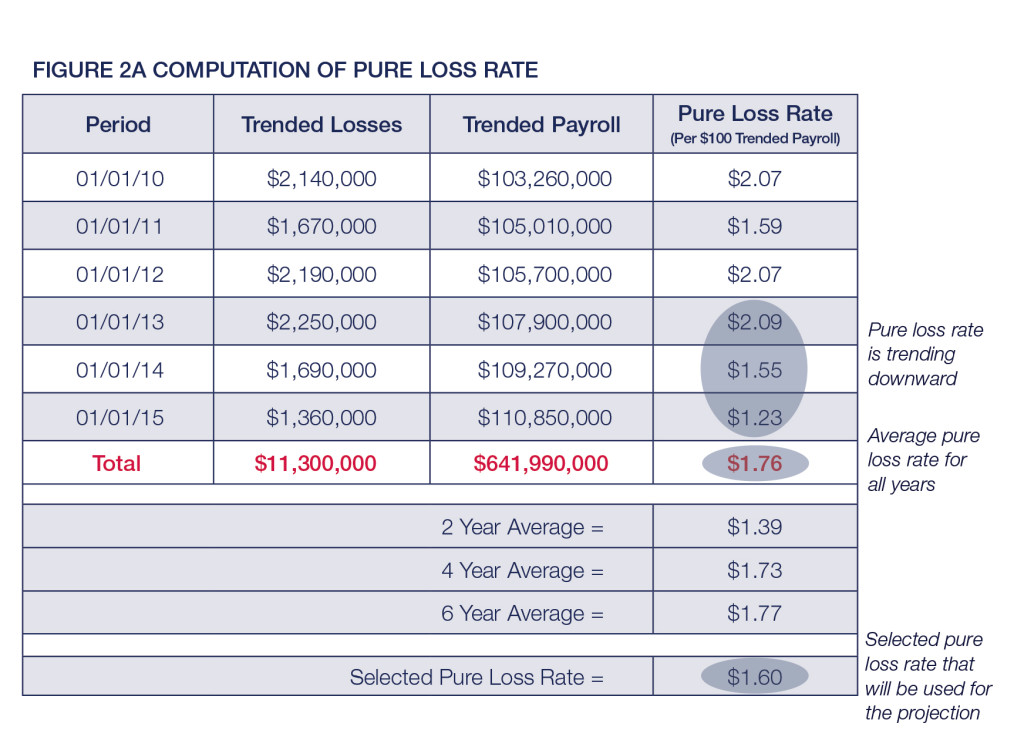
The next step is to calculate pure loss rates based on the historical experience. This procedure uses past experience to determine a factor which, when applied to payroll, produces an estimate of ultimate incurred losses. In this case, the pure loss rate can be defined as the expected dollar loss cost per $100 of payroll. Trended losses are divided by trended exposures to yield pure loss rates based on the unique experience of each historical period. Each of the calculated pure loss rates is an estimate of the pure loss rate which could be charged for the projected period. A pure loss rate of $1.60 per $100 has been selected for the projected period. This is shown in Figure 2a.

Sample Case – Making the Projection

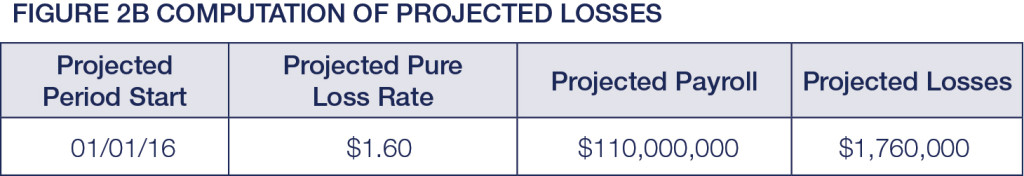
Finally, the selected pure loss rate of $1.60 per $100 of payroll is multiplied by the projected payroll to forecast losses of $1,760,000, an amount often referred to as the loss pick. This final computation is shown in Figure 2b.

Up to the point of selecting the pure loss rate for the forecast, the process is pure mathematics using historical data and trending factors. However, the selection of the pure loss rate involves judgment. This is where good communication with the actuary is critical to attaining the most accurate projection possible. The actuary has full access to the objective historical data, but subjective information pertaining to changes in business operations, safety programs, new product introductions, changes in manufacturing techniques, or other pertinent conditions may affect the selected pure loss rate. This is especially important when a “bad” year with a higher pure loss rate skews perception of recent history.

In Figure 2a, average rates for two, four, and six years are shown. The most recent two years show a significant trend downward in the pure loss rates. After discussions concerning new loss prevention programs that the client recently established, the actuary selected a pure loss rate of $1.60. This is lower than the average $1.76 and gives more weight to the recent years' experience.

We welcome your feedback by posting a comment, or contact me at  TLC@SIGMAactuary.com.