The projection of losses involves estimating the expected or average value of future loss costs. This estimate is based on historical loss experience, adjusted to the current cost level considering both internal influences (such as development, changes in claims reserving, exposure volume and mix of business) and external influences (such as inflation and changes in the judicial, legislative and regulatory environment).

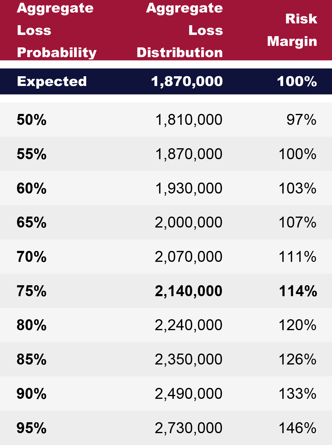
This point estimate provides the basis for understanding the average loss cost involved with retaining losses. A confidence level analysis takes this one step further by quantifying the variance around the point estimate and the additional risk involved with retaining losses. This variance, in a typical SIGMA analysis, is presented as a list of projected loss values and the probability of actual losses falling above or below each value.

For example, in the following table projected losses are $1,870,000 on an expected basis or for an average year. However, 75% of the time (3 out of 4 years) losses are anticipated to be up to $2,140,000. This loss amount is approximately 14% above the expected value. When funding for an upcoming year, choosing a level higher than the expected value increases the ability of a program to withstand losses greater than anticipated. This type of analysis is useful for comparing the risk involved with different risk retention and transfer options, such as varying per occurrence and aggregate retentions or combining multiple risks into a single program.

Similar to the expected loss projection, estimates at each confidence level rely primarily on historical loss experience. Loss severity and claim count distributions are chosen considering the historical loss experience with the intention of quantifying any gaps in the history. Thus, several assumptions regarding appropriate distributions and parameters must be made. It is important for decision makers to understand these assumptions and discuss with their actuary any potential events which may not be captured historically. Actuarial judgment and qualitative information should be considered, alongside the qualitative information, during this process.

For example, the loss history may not fully represent the future situation. Using a short-term loss history to determine the severity distribution may not capture potential shock losses or catastrophes. The COVID-19 pandemic is an example of losses not captured in the short or even long-term history. The resulting loss implications on say workers compensation, whether in a high-risk industry such as healthcare or lower-risk industry adapted to new work-from-home environments, are still unfolding. Additionally, the judicial environment for liability claims is evolving and the future situation may not be captured by relying solely on historical experience.

The statistical distribution and associated parameters may not represent the full range in future values. For example, a chosen severity distribution may have a good fit for higher loss severities (in the tail) but not for lower severities or vice versa. This may produce inaccurate estimates when comparing a program with a lower retention level to a program with a higher retention level. It is important for the actuary to understand the intended use of the analysis, in order to determine any items which may have a material impact on the results and discuss these implications with those relying on the results.

SIGMA actuaries are available to discuss the use of confidence level analyses unique to your particular program and any limitations present in the unique data. Additional resources are available at RISK66.com.

If you are not currently a RISK66 subscriber, sign up for our complimentary Education License.

We welcome your feedback by posting a comment or contacting us at support@SIGMAactuary.com.

© SIGMA Actuarial Consulting Group, Inc.